This morning, I just found out about #tidytuesday and I figured it would be a fun thing to play with.
For my first foray into tidytuesday, we have data on Bob Ross’s paintings during his show. The data were compiled by fivethirtyeight and reported here.
The data are available here. On the info page for the data, they show how to load the data and give an example of some basic tidying. I’ll do that below:
library(dplyr)
library(tidyr)
library(stringr)

bob_ross <-
  readr::read_csv("https://raw.githubusercontent.com/rfordatascience/tidytuesday/master/data/2019/2019-08-06/bob-ross.csv")

# to clean up the episode information
bob_ross <-
  bob_ross %>%
  janitor::clean_names() %>%
  separate(episode, into = c("season", "episode"), sep = "E") %>%
  mutate(season = str_extract(season, "[:digit:]+")) %>%
  mutate_at(vars(season, episode), as.integer)

head(bob_ross)
## # A tibble: 6 x 70
## season episode title apple_frame aurora_borealis barn beach boat bridge
## <int> <int> <chr> <dbl> <dbl> <dbl> <dbl> <dbl> <dbl>
## 1 1 1 "\"A… 0 0 0 0 0 0
## 2 1 2 "\"M… 0 0 0 0 0 0
## 3 1 3 "\"E… 0 0 0 0 0 0
## 4 1 4 "\"W… 0 0 0 0 0 0
## 5 1 5 "\"Q… 0 0 0 0 0 0
## 6 1 6 "\"W… 0 0 0 0 0 0
## # … with 61 more variables: building <dbl>, bushes <dbl>, cabin <dbl>,
## # cactus <dbl>, circle_frame <dbl>, cirrus <dbl>, cliff <dbl>,
## # clouds <dbl>, conifer <dbl>, cumulus <dbl>, deciduous <dbl>,
## # diane_andre <dbl>, dock <dbl>, double_oval_frame <dbl>, farm <dbl>,
## # fence <dbl>, fire <dbl>, florida_frame <dbl>, flowers <dbl>,
## # fog <dbl>, framed <dbl>, grass <dbl>, guest <dbl>,
## # half_circle_frame <dbl>, half_oval_frame <dbl>, hills <dbl>,
## # lake <dbl>, lakes <dbl>, lighthouse <dbl>, mill <dbl>, moon <dbl>,
## # mountain <dbl>, mountains <dbl>, night <dbl>, ocean <dbl>,
## # oval_frame <dbl>, palm_trees <dbl>, path <dbl>, person <dbl>,
## # portrait <dbl>, rectangle_3d_frame <dbl>, rectangular_frame <dbl>,
## # river <dbl>, rocks <dbl>, seashell_frame <dbl>, snow <dbl>,
## # snowy_mountain <dbl>, split_frame <dbl>, steve_ross <dbl>,
## # structure <dbl>, sun <dbl>, tomb_frame <dbl>, tree <dbl>, trees <dbl>,
## # triple_frame <dbl>, waterfall <dbl>, waves <dbl>, windmill <dbl>,
## # window_frame <dbl>, winter <dbl>, wood_framed <dbl>There are a couple of paintings that are named the same thing.
bob_ross <-
  bob_ross %>%
  group_by(title) %>%
  mutate(title_count = 1:group_size(.)) %>%
  ungroup() %>%
  mutate(title = if_else(title_count > 1,
                         paste(title, title_count),
                         title)) %>%
  select(-title_count)
There are some columns that are relate to the frame the painting got put into and some columns that relate to elements inside each painting. Like the fivethirtyeight crew, I’m more interested in the elements inside the paintings as opposed to the frames, so i’ll go ahead and drop those columns
painting_data <-
  bob_ross %>%
  select(-contains("frame"), -steve_ross, -guest, -diane_andre)
In my professional work, I perform social network analysis, so let’s go ahead and look at networks of elements in Bob Ross’s paintings!
Networks of Bob Ross Paintings
To get us looking at social networks, we first need to take the data from this wide format and turn it into an edge list. The edge list will connect each painting to every element that is inside it. From there, we can get a picture of what the network of paintings looks like!
Organizing the Edge List
library(igraph)
library(ggnetwork)

titles <- painting_data[["title"]]
incidence_mat <-
  painting_data %>%
  select(-season, -episode, -title)

incidence_mat <- as.matrix(incidence_mat)
rownames(incidence_mat) <- titles

incidence_graph <-
  graph_from_incidence_matrix(incidence_mat, )

ggplot(incidence_graph, aes(x = x, y = y, xend = xend, yend = yend)) +
  geom_edges() +
  # type is TRUE if a node is an episode and FALSE if it's an element
  geom_nodes(aes(color = type)) +
  theme_blank()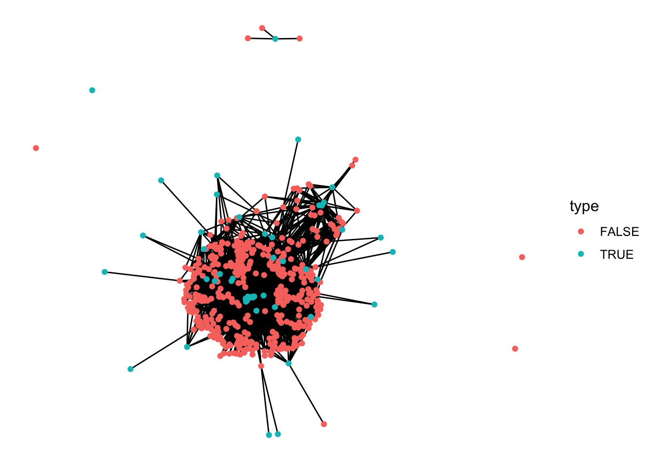
That’s real busy! It looks like there are a few episodes that only have a few elements and some episodes that have many elements in it. There’s also that one episode that shares three elements with another episode and no others.
Let’s see if we can clean this up a bit! First, i’ll connect episodes by how many elements they share.
episode_x_episode <- incidence_mat %*% t(incidence_mat)

ep_x_ep_graph <-
  graph_from_adjacency_matrix(episode_x_episode,
                              # only look at the upper part of the matrix since it is symetrical
                              mode = "upper",
                              # the connections are weighted
                              weighted = TRUE,
                              # don't count self-loops
                              diag = FALSE)

ggnetwork(ep_x_ep_graph, weight = "weight") %>%
  ggplot(aes(x = x, y = y, xend = xend, yend = yend)) +
  geom_edges() +
  geom_nodes() +
  theme_blank()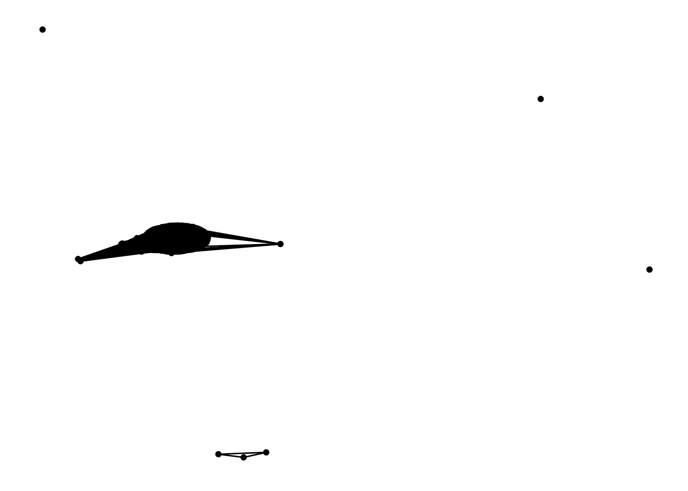
Not much to look at. Or better yet, Ross’s paintings tend to share something in common with other paintings.
Instead of looking at all the features at once, why don’t we look at groups of features. I’ve gone ahead and grouped each feature into different categories. I’ll load that up and then split up the painting df into different categories.
feature_categories <-
  readr::read_csv("../../data/Bob Ross/ross_painting_features.csv")

painting_categories <-
  painting_data %>%
  gather(feature, value, -season, -episode, -title) %>%
  left_join(feature_categories, by = "feature") %>%
  filter(value > 0) %>%
  count(season, episode, title, category) %>%
  spread(category, n) %>%
  mutate_at(vars(-season, -episode, -title), ~if_else(is.na(.), 0, 1))

titles <- painting_categories[["title"]]


incidence_mat <-
  painting_categories %>%
  select(-season, -episode, -title) %>%
  as.matrix()
rownames(incidence_mat) <- titles

episode_x_episode <- incidence_mat %*% t(incidence_mat)


ep_x_ep_graph <-
  graph_from_adjacency_matrix(
    episode_x_episode,
    # only look at the upper part of the matrix since it is symetrical
    mode = "upper",
    # the connections are weighted
    weighted = TRUE,
    # don't count self-loops
    diag = FALSE)

# add in season as an attribute of each episode
vertex_attr(ep_x_ep_graph, "season") <- painting_categories[["season"]]
Now to plot! I’m going to build these plots with a cutpoint though, because otherwise they become very unweildy.
ep_x_ep_graph %>%
  delete_edges(which(edge_attr(ep_x_ep_graph)$weight <= 2)) %>%
  delete_vertices(., which(igraph::degree(.) == 0)) %>%
  ggnetwork(weight = "weight") %>%
  ggplot(aes(x = x, y = y, xend = xend, yend = yend)) +
  geom_edges(color = "gray") +
  geom_nodes(aes(color = season)) +
  theme_blank() +
  Friedman::scale_color_drexel(discrete = FALSE) +
  labs(title = "Paintings that share 3, 4, or 5 feature categories")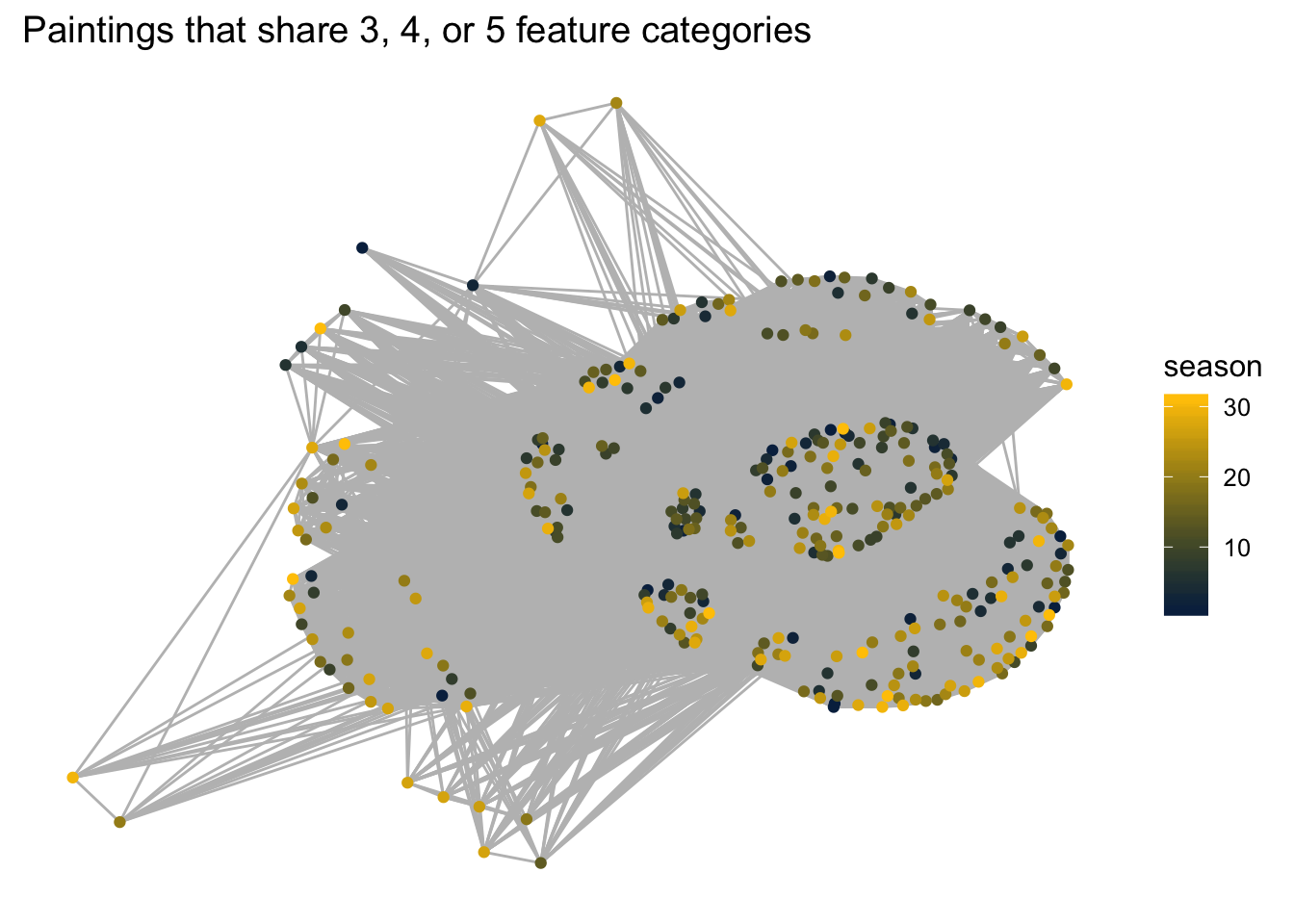
Above, I’ve colored nodes by season and only shown connections between episodes if those episodes share more than two classes of feature (e.g. two episodes have a sky feature, tree and plant feature, and a man-made feature).
What happens if we filter to only show edges if two espodes share 4 features? 5?
 Looking at the paintings that share more than 3 features really brings about that there is a central group of paintings that all share a lot in common and then a few different groups of paintings that all have different things in common.
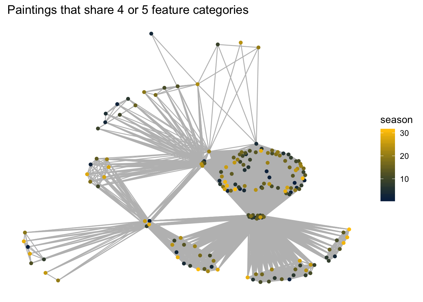
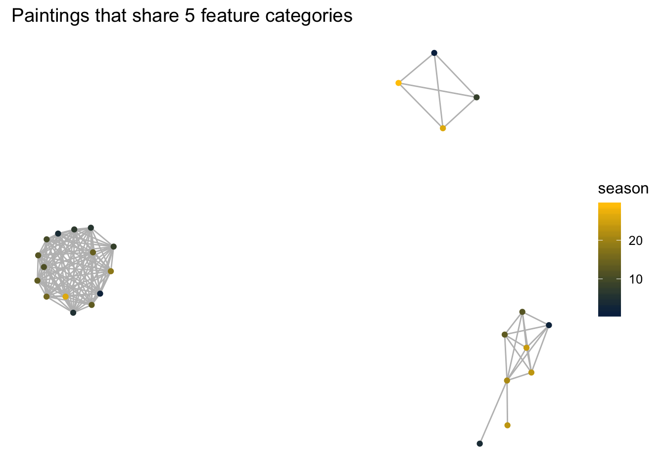
Now looking just at paintings that share 5 feature categories, it can really be seen that there is a central set of themes that is very common accross seasons. What are they?
episodes_of_interest <-
  ep_x_ep_graph %>%
  delete_edges(which(edge_attr(ep_x_ep_graph)$weight <= 4)) %>%
  delete_vertices(., which(igraph::degree(.) == 0)) %>%
  vertex_attr("name")

painting_categories %>%
  filter(title %in% episodes_of_interest) %>%
  mutate(feature_sum = aquatic + clouds + `general nature` +
           `man made` + nature + sky + `trees and plants`) %>%
  filter(feature_sum > 4) %>%
  summarize_at(vars(-season, -episode, -title, -feature_sum), sum)
## # A tibble: 1 x 7
## aquatic clouds `general nature` `man made` nature sky `trees and plant…
## <dbl> <dbl> <dbl> <dbl> <dbl> <dbl> <dbl>
## 1 27 23 27 19 3 11 26All (or near all) of these paintings have an aquatic element, a general nature element, and trees and plants. So the real defining factor between the three groups in the plot above probably has to do with the other four categories. Next time I play with these data, I’ll look at that and do a deeper dive on components of the network of Bob Ross paintings.